STREAM Help

What is STREAM

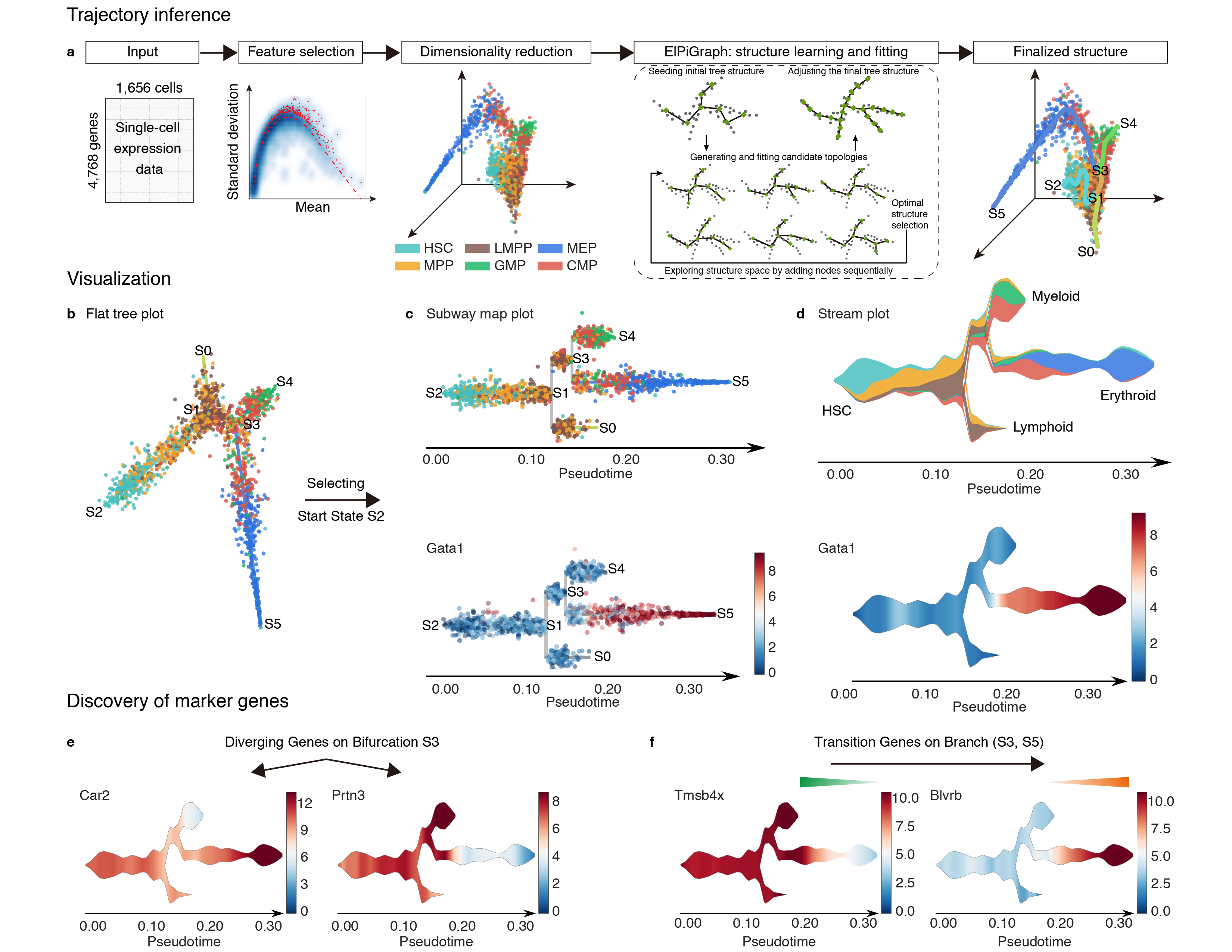
STREAM(Single-cell Trajectories Reconstruction, Exploration And Mapping of omics data), is an interactive pipeline capable of disentangling and visualizing complex branching trajectories from both single-cell transcriptomic and epigenomic data. It also allows for automatic developmental-trajectory-related marker gene discovery and visualization.

STREAM is available as user-friendly open source software and can be used interactively as a web-application at stream.pinellolab.org or as a standalone command-line tool with Docker https://github.com/pinellolab/STREAM

What can I do with STREAM

STREAM can be used in two different ways:

1. An interactive database focused on single-cell trajectory visualization for several published studies.

Users can visualize and explore cells’ developmental trajectories, subpopulations and their gene expression patterns at single-cell level.

2. A computational trajectory inference tool:

• STREAM can take as input both single cell transcriptomic and epigenomic data. It reliably reconstructs trajectories and pseudotime in both simple bifurcation or complex branching situation without the need of prior knowledge about the structure or the number of trajectories


• STREAM provides the mapping procedure, which permits reusing a previously inferred principal graph as reference to map new cells not included in the original fitting procedure (Currently it's only supported at command line interface https://github.com/pinellolab/STREAM)


• STREAM provides analytical tools for potential marker genes (or k-mers) of different types: diverging genes, i.e. genes important in defining branching points that are differentially expressed between diverging branches, and transition genes, i.e. genes for which the expression correlates with the cell pseudotime on a given branch.


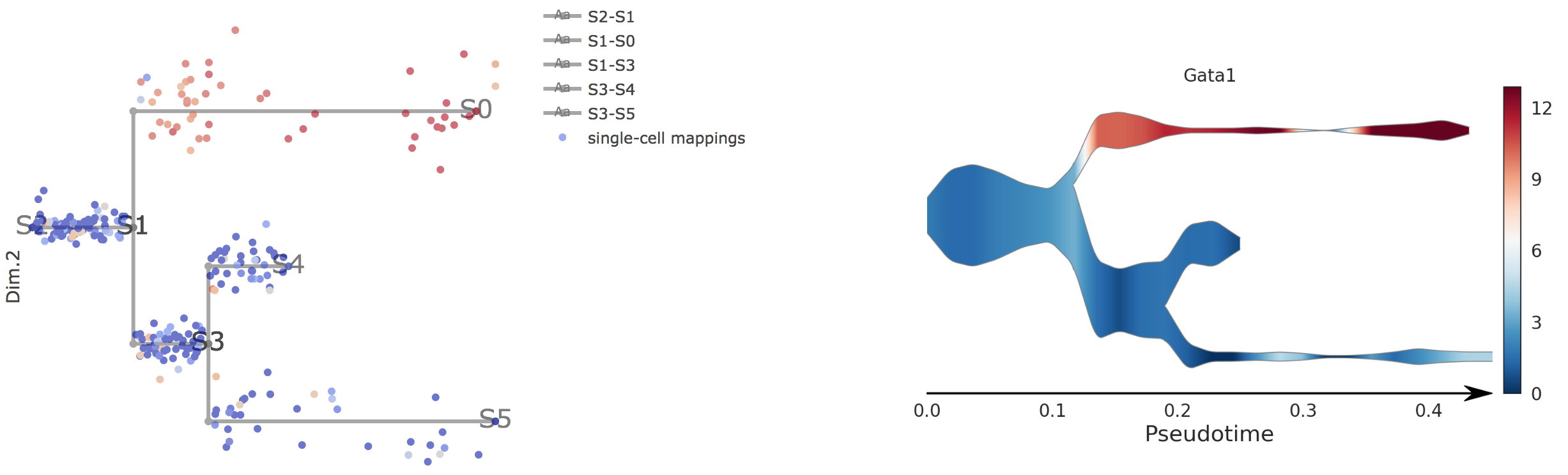
• STREAM provides both single-cell-level and density-level visualizations of cells and gene expression patterns for inferred trajectories. Specially, STREAM proposed a novel visualizaiton, called the stream plot, which is useful to study subpopulation composition and cell-fate genes along branching trajectories

Usage

1.Precomputed results:

By clicking on 'Precomputd resutls', users are able to visualize precomputed trajectories for several published datasets. (More datasets will be included in future)

1).Choose Precomputed Data Set

Users can choose any precomputed data from the droplist. Here we take 'Guo,G.et al.2013' as an example:
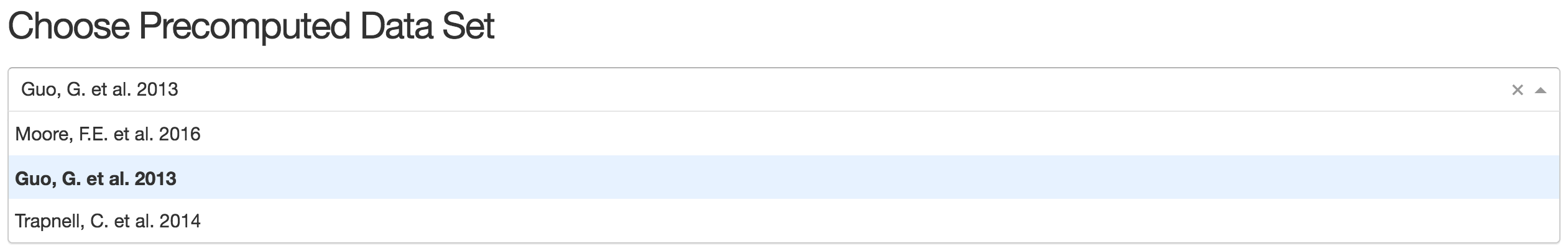
once user chose the dataset, a brief description will automatically appear beneath the menu.

2).Visualize Trajectories

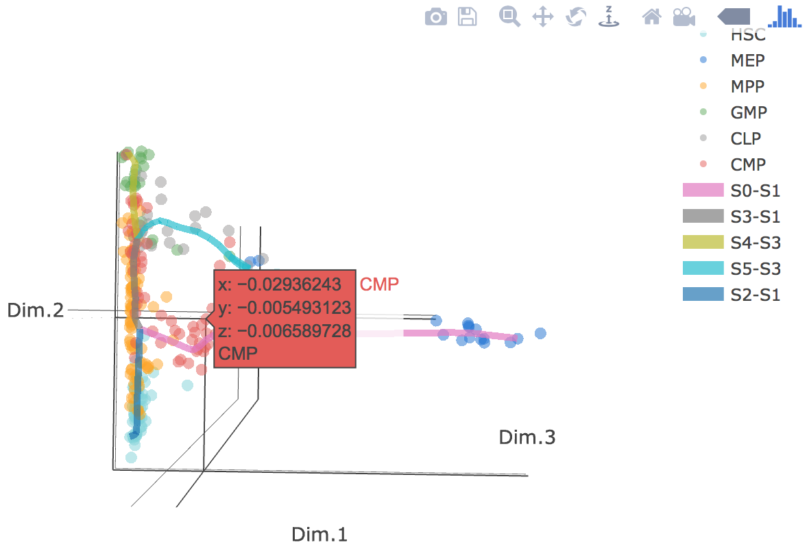
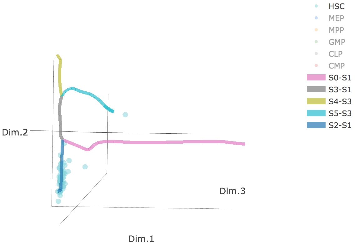
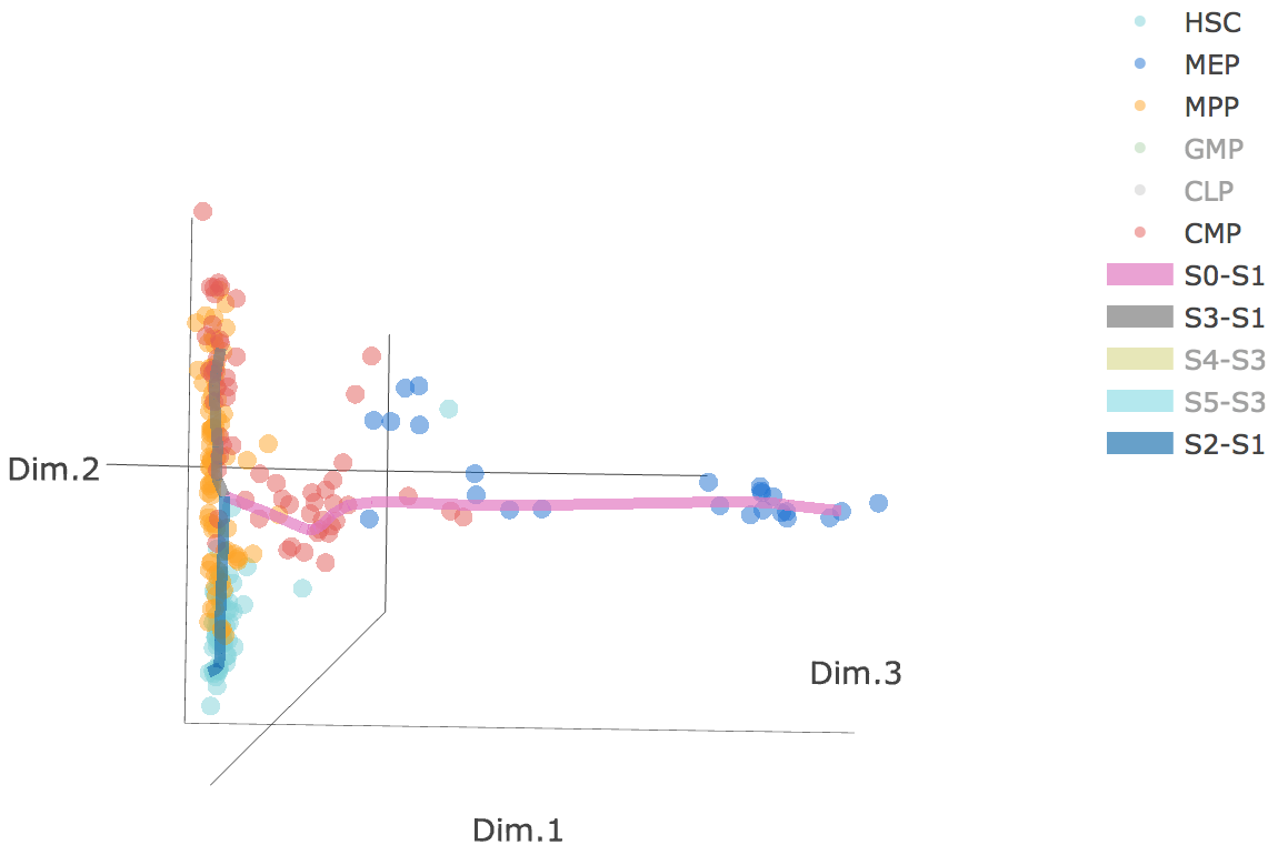
3D scatter plot shows cells' positions and fitted principal graph by STREAM in MLLE space. In the 3D scatter plot, users can easily and interatively perform a lot of different operations including rotatation, zoom-in, zoom-out, taking snapshots at a specific view.



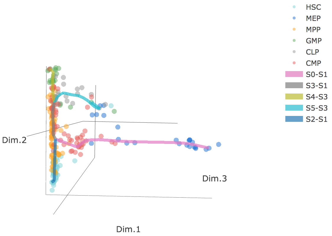
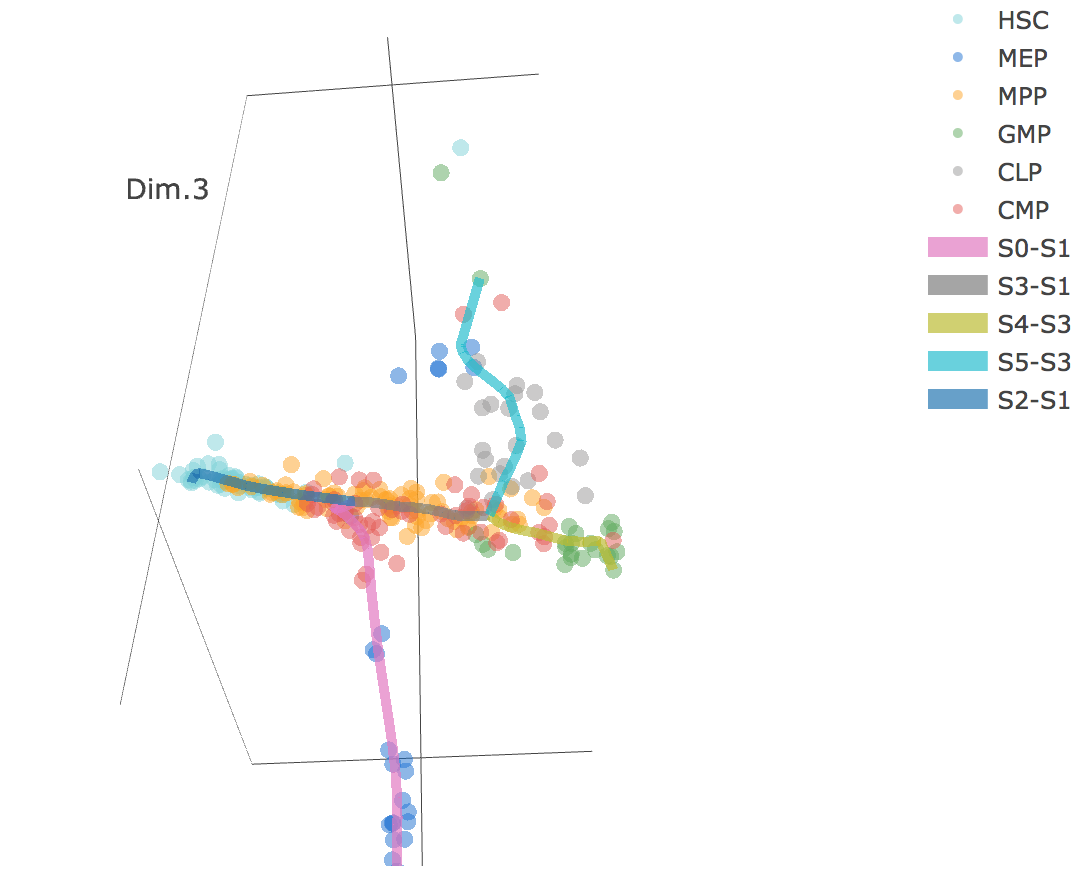
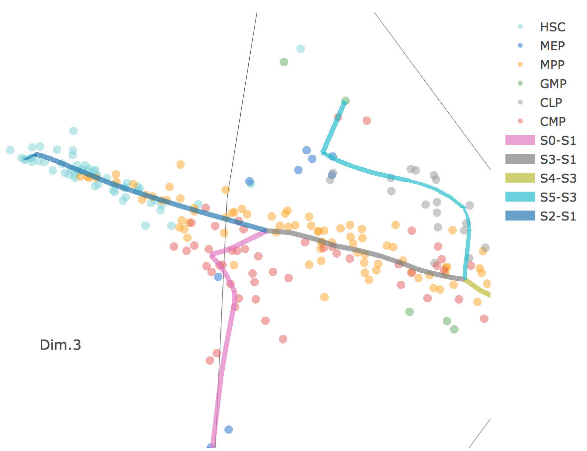
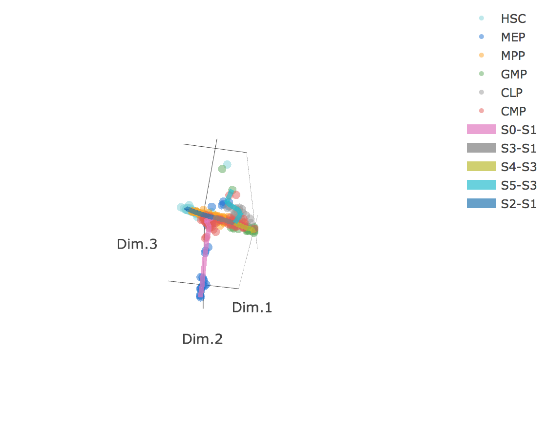
Additionally, when hovering the mouse over points, cells' coordinates and cell labels obtained from experiment will show up. Users can also interactively control the legend panel. By clicking on cell type or fitted curve first time, the related cells or curves will disppear. By clicking them again, cells or curves will come back. This helps focus on branch or cell type of interest.


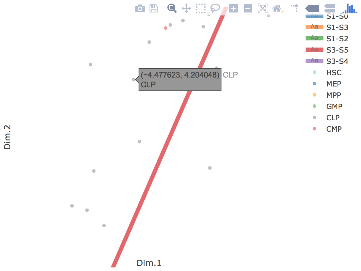
Flat tree plot intuitively and conveniently represents curves(trajectories) as linear segments in a 2D plane. In this representation, the lengths of tree branches are preserved from three or higher dimenional MLLE space. In addition, cells are projected onto the tree according to their branch locations and the distances from their assigned branches. When hovering the mouse over points, cells' coordinates in 2D plane and cell labels obtained from experiment will appear. Users can zoom in by selecting a specific area. Similar to 3D scatter plot, users can interactively control the legend part.



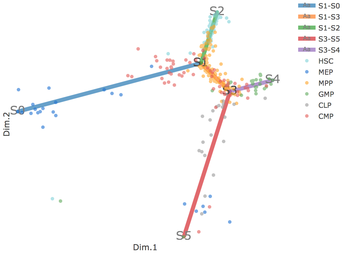
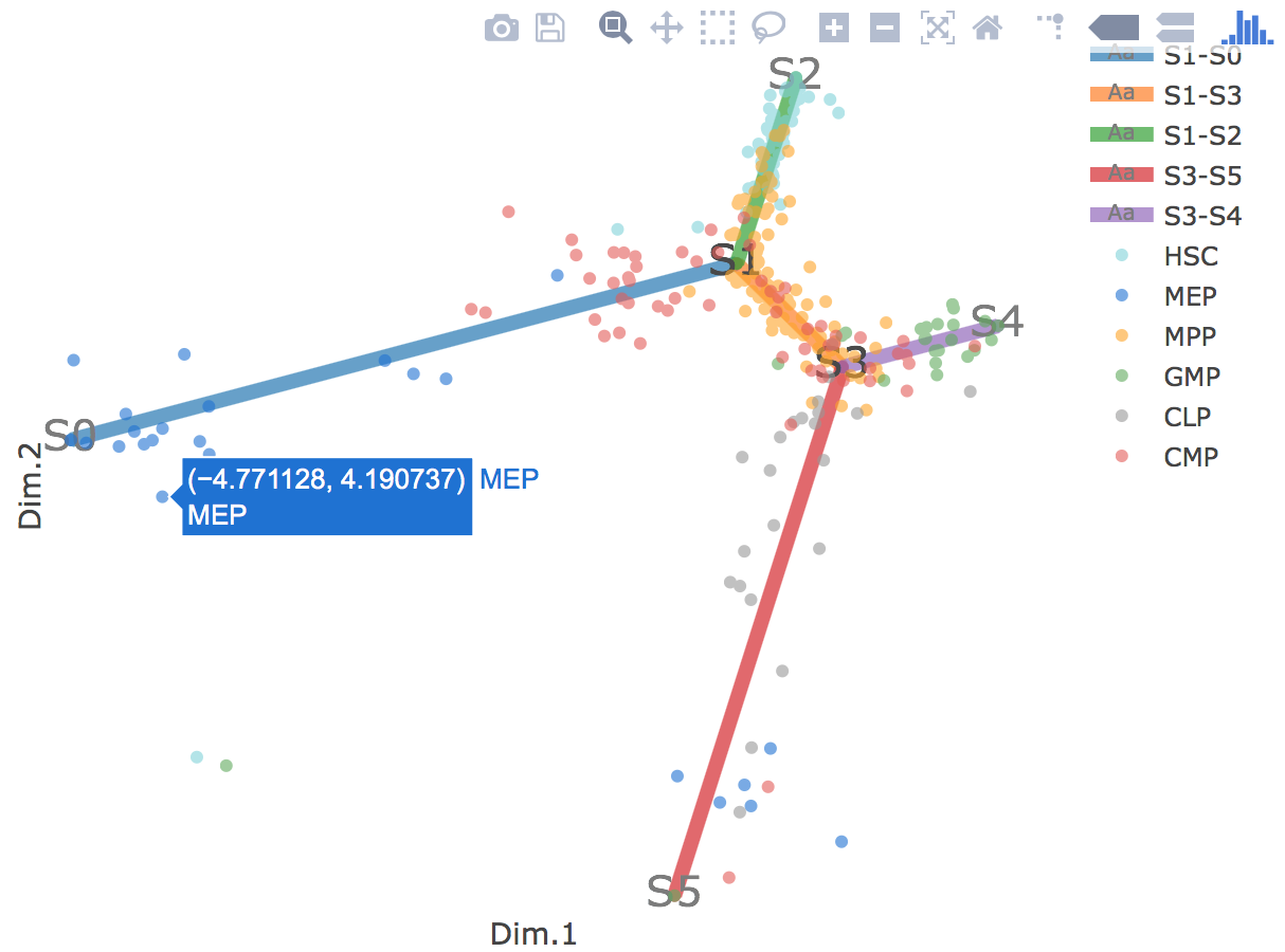
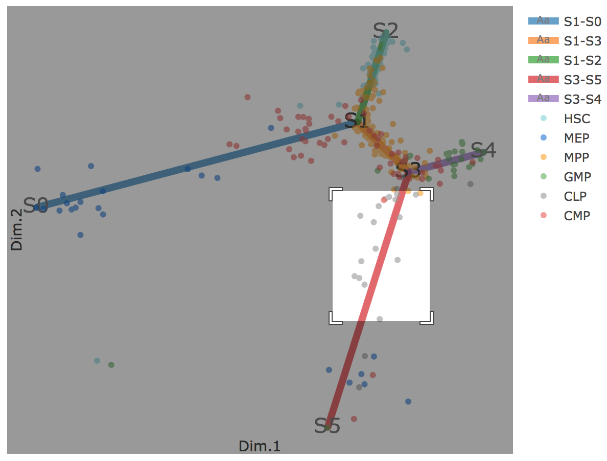
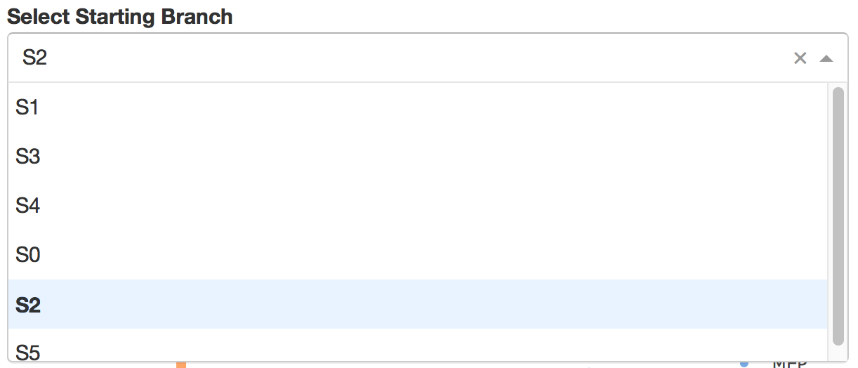
Users can select different starting nodes to visualize the trajectories in subway map (at single-cell level) or stream plot (at density level). By default, the recommended start node is selected. This allows easily re-organization of the tree using breadth-first search to better represents pseudotime progression from a selected starting node.



3).Visualize Genes of Interest

In the gene combo box,users can either choose genes from the droplist or type in gene name themselves.

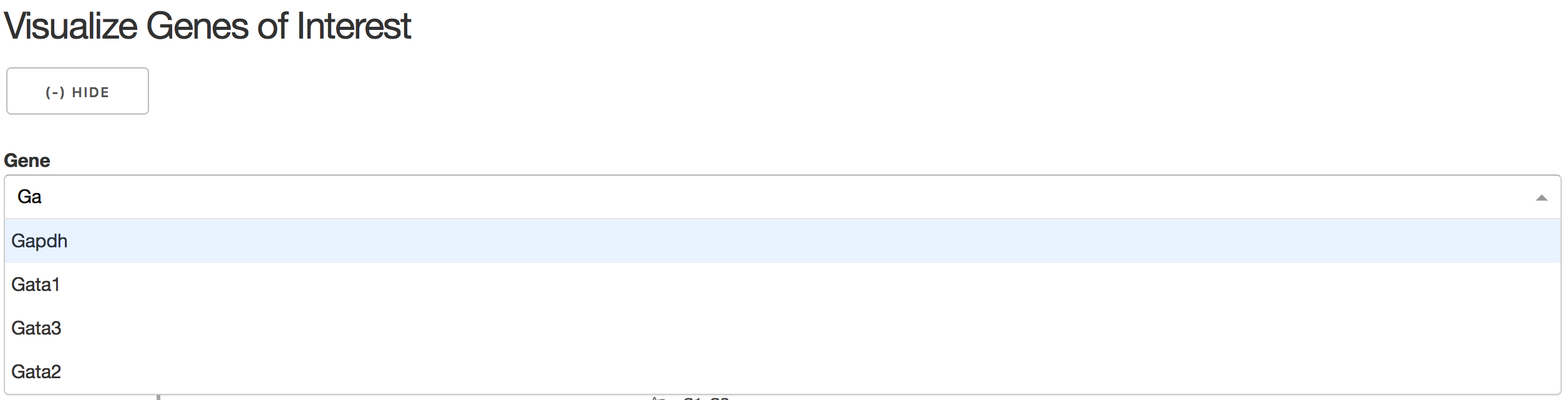
Genes will be visualized in both subway map and stream plot. When hovering the mouse over point, both cells' coordinates and gene expressions will be displayed.


4).Visualize Diverging Genes

Diverging genes, i.e. genes important in defining branching points that are differentially expressed between diverging branches.
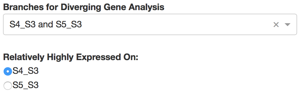
Users first need to choose a pair of adjacent branches, between which differentially expressed genes were calculated by STREAM.

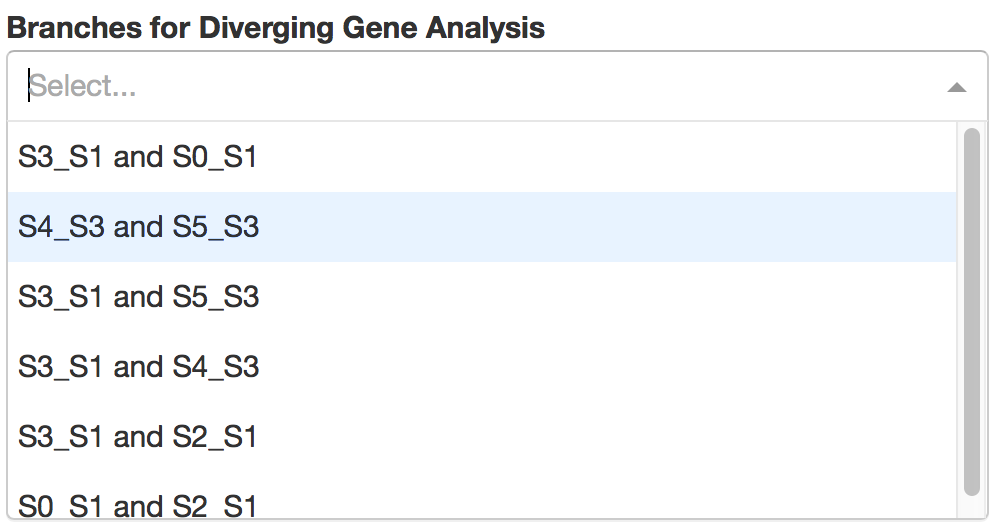
Then users can specify the branch on which DE genes are relatively highly expressed.

Top automatically detected DE genes will be showned. Users can easily control how many genes to display through a slider bar.

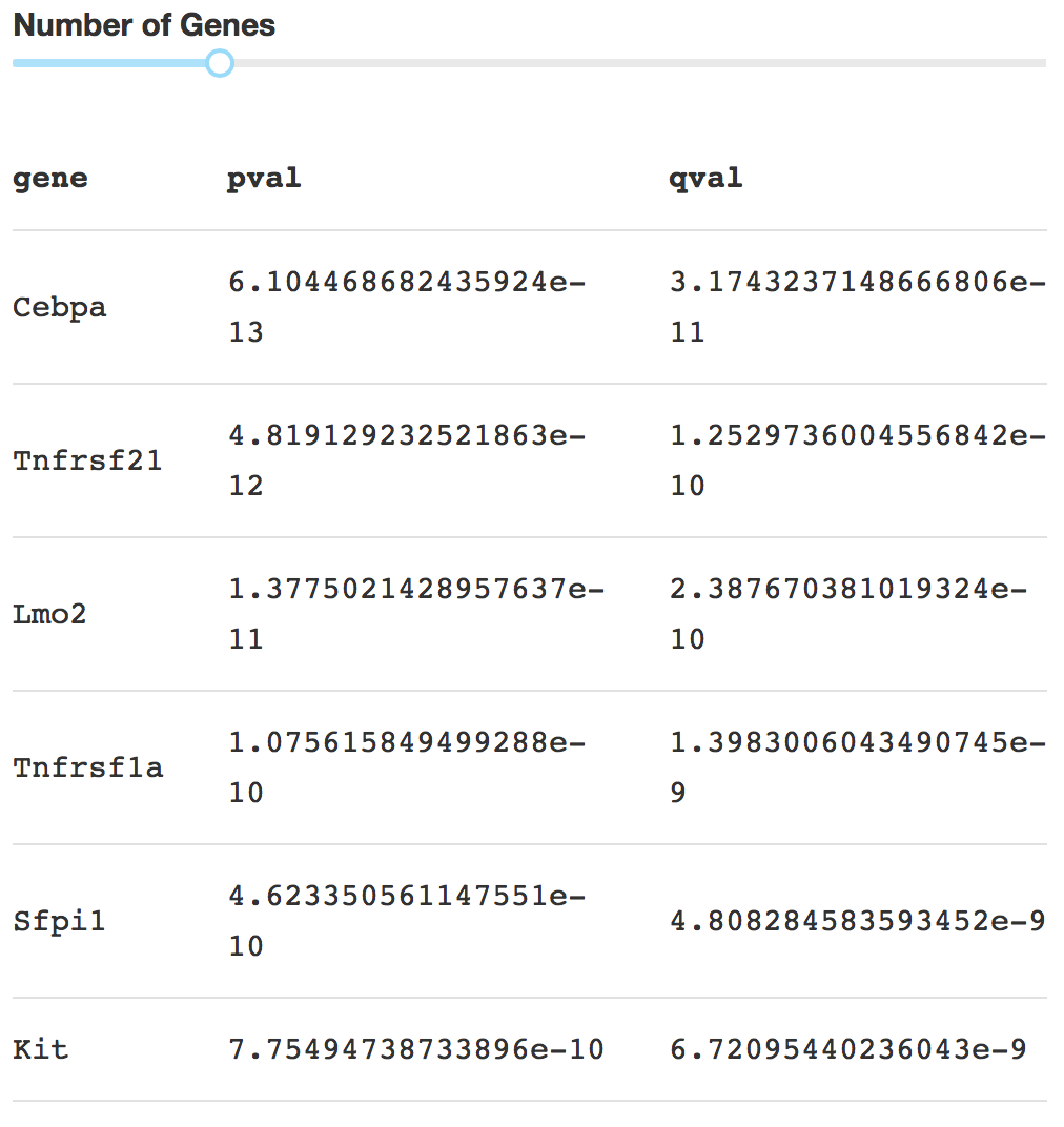
On the right, users can visualize detected diverging gene at flat tree and stream plot.

5).Visualize Transition Genes

Transition genes, i.e. genes for which the expression correlates with the cell pseudotime on a given branch.
Users first need to choose one branch, along which transition genes were calculated by STREAM.

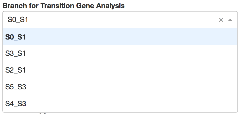
Then top automatically detected transition genes will be displayed. Users can easily control how many genes to display through a slider bar.

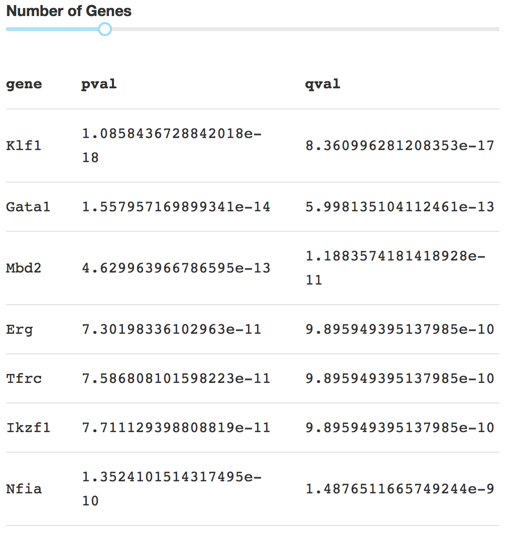
On the right, users can visualize detected transition gene.

2.Compute on your own data:

1).Input files

Data Matrix:
For transcriptomic data, STREAM only requires a tab-separated gene expression matrix (raw counts or normalized values) in .tsv or .tsv.gz file format. Each row represents a unique gene and each column is one cell. For raw counts, log2 transformation and library size normalization are necessary.

	HSC1	HSC1.1	HSC1.2	HSC1.3	HSC1.4
CD52	6.479620	0.000000	0.000000	5.550051	0.000000
Ifitm1	11.688533	11.390682	10.561844	11.874295	8.976571
Cdkn3	0.000000	0.000000	0.000000	0.000000	8.293616
Ly6a	10.417026	11.452145	0.000000	8.158840	8.945882
Bax	6.911608	10.201157	0.000000	9.396073	0.000000


For epigenomic data, to perform scATAC-seq trajectory inference analysis, the main input can be:
1)a set of files including count file, region file and sample file. Since this part is a bit time-consuming, currently it's not supported by the website yet. But users can easily achieve it by running STREAM at command line interface https://github.com/pinellolab/STREAM.
2)a precomputed scaled z-score file by STREAM. Each row represents a k-mer DNA sequence. Each column represents one cell. Each entry is a scaled z-score of the accessibility of each k-mer across cells

	singles-BM0828-HSC-fresh-151027-1	singles-BM0828-HSC-fresh-151027-2	singles-BM0828-HSC-fresh-151027-3
AAAAAAA	-0.15973157637808505	0.18950966450007853	0.07713107176524692
AAAAAAG	-1.3630723054479532	-0.04770034004421244	0.6387323857481045
AAACACG	-0.2065161126378667	-1.3375384076872765	0.2660278729402342
AGCGTTA	-0.496859947462221	0.7181918229050274	0.19603357892921522
ATACTCA	-1.2127919166377426	0.7938414496478844	-1.2665513250104594




Additionally it is possible to provide these following files in .tsv or .tsv.gz format:
cell_labels file: .tsv or .tsv.gz format. Each item can be a putative cell type or sampling time point obtained from experiments. Cell labels are helpful for visually validating the inferred trajectory. The order of labels should be consistent with cell order in the gene expression matrix file. No header is necessary.

HSC

HSC

GMP

MEP

MEP

GMP


cell_label_color file: .tsv or .tsv.gz format. Customized colors to use for the different cell labels. The first column specifies cell labels and the second column specifies the color in the format of hex. No header is necessary.

HSC	#7DD2D9
MPP	#FFA500
CMP	#e55b54
GMP	#5dab5a
MEP	#166FD5
CLP	#989797

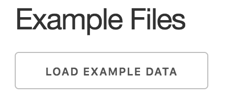
In addition to personal files, in order to help users quickly get an idea how STREAM works, users can simply click the button 'load example data'. This will automatically upload data matrix file,cell_labels file and cell_label_color file for users.


2).Parameters

This panel mainly consists of basic parameters and advanced parameters. The basic parameters should be able to work well in most cases. It's necessary to do log2 transformation and library size normalization if the data matrix provided by user contains raw count. Also since scATAC-seq data is very different from transcriptomic data, users need to specify whether it's ATAC-seq data or not. For feature selection, by default, we use LOESS fitting to select most variable genes. In scATAC-seq data, because z-score matrix has negative values, users need to use PCA to select top PCs. In sc-qPCR data,usually the number of gene is relatively small, we suggest that users keep all the genes by choosing 'all'. For dimension reduction, we are using MLLE. The neighbor size is chosen based on the number of cells and is set by default to 10% of the total number of cells. The number of MLLE components to use depends on the number of branches and on the complexity of the structure to learn. Typically, three components capture the main structure for most datasets, increasing them may recover finer structures (although we observed that there is no benefit for selecting more than 5 components in all the datasets tested).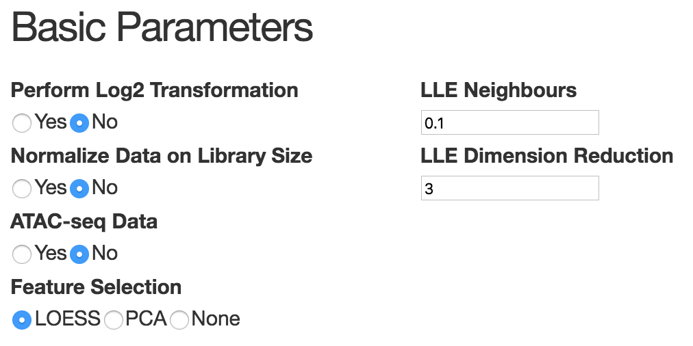


3).Compute Trajectories

When users click the button "compute", STREAM will infer trajectories based on the parameters set by users. The process may take a few minutes depending on the data size (For sc-qPCR data with hundreds of cell, it may take one minute. For scRNA-seq data with around 2000 cells and 3k genes, it may take two minutes). Once it's done, similar to the part "precomputed results", users are able to see different interactive visualizations including 3D scatter plot with fitted trajecotries, flat tree plot, subway map and stream plot. For subway map and stream plot, users can explore different re-organizations of the inferred tree structure by choosing different start node.

4).Visualize Genes of Interest

Similar to the 'Precomputed results', after choosing the gene of insterst, users can simply click "perform analysis" to interactively visualize its gene expression pattern in both subway map and stream plot obtained from the step 'Compute trajectories'.

5).Identify Diverging Genes

Users can simply click the button 'perform analysis' and start the diverging genes analysis. Then the button status will become 'running'. This process usually takes longer than 'compute trajectories'. The running time varies depending on the number of genes and cells. (For sc-qPCR data with hundreds of cell, it may take around five minutes. For scRNA-seq data with around 2000 cells and 3k genes, it may take around eight minutes). Once it's completed, similar to 'Precomputed results', diverging gene will be displayed based on the pair of branches users have choosen and users can interactively visualize diverging genes in subway map and stream plot on the right.

6).Identify Transition Genes

Users can simply click the button 'perform analysis' and start the transition genes analysis. Then the button status will become 'running'. This process usually is a little faster than diverging genes analysis (For sc-qPCR data with hundreds of cell, it may take around three minutes. For scRNA-seq data with around 2000 cells and 3k genes, it may take around six minutes). Once it's completed, similar to 'Precomputed results', transition gene will be displayed based on specific branch users have choosen and users can interactively visualize transition genes in subway map and stream plot on the right.

Download current analysis

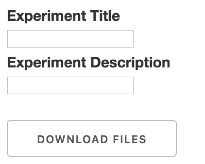
Having finished the previous analysis steps, by clicking 'download files', users can easily download STREAM analyis results. All the results will be formalized and included in a zip file. Users are also more than welcome to provide to us their personal analysis results from STREAM. We will be happy to include that in the precomputed results part on STREAM website.(For 3D scatter plot,flat tree plot and subway map, users can also easily download them directly from the interactive plots)